Is an LLM Deterministic or Probabilistic? A Deep Dive into Softmax & Co.

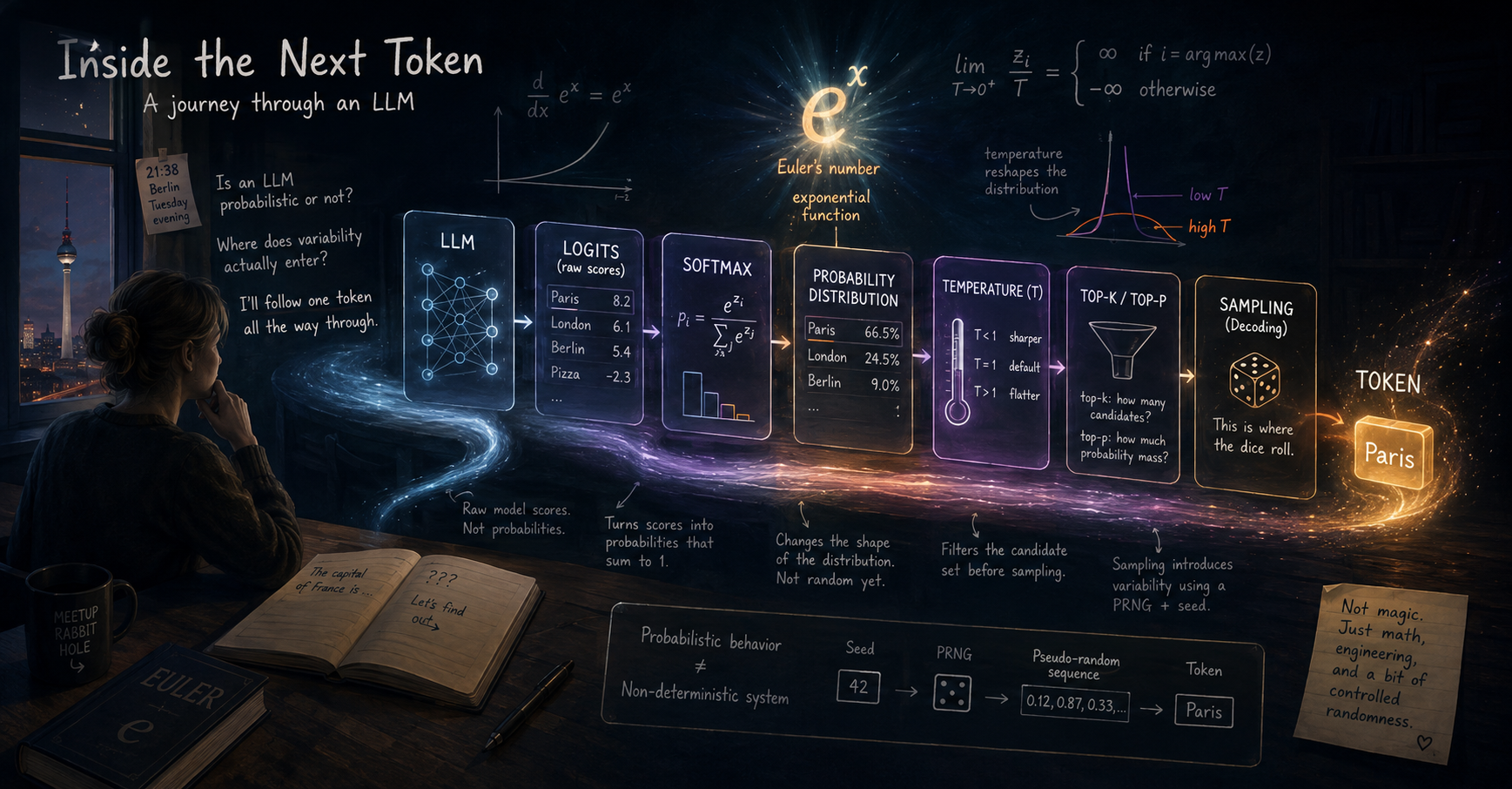
Euler’s night

21:38. Berlin. Tuesday evening.

I had just come home from a meetup with a question in my head. (Btw, thanks Sergiusz and Stefan for your fantastic talk … and the rabbit hole!)

Is an LLM probabilistic or not?

Because, well… somehow yes. But also somehow no. So I decided to follow one token all the way through the system.

What actually happens between „the model predicts a token“ and „the model produces a token“?

In summary, an LLM first scores every possible next token. Softmax turns those scores into a probability distribution. A decoding strategy then decides whether to select the most likely token or sample one according to those probabilities.

---

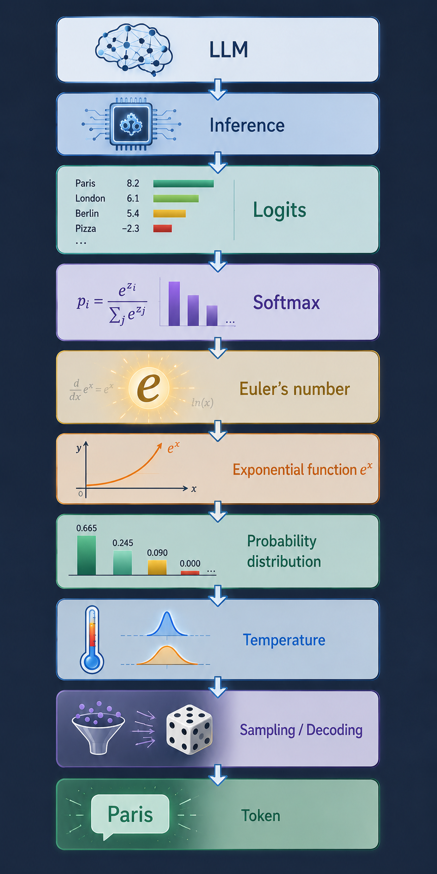
So, what happens when an LLM generates a token?

When an LLM processes a prompt, it does not simply decide: „The next token is Paris.“ First of all, the model takes the input and produces a score for every possible next token, based on its learned weights.

Suppose the context is:

The capital of France is …

Conceptually, the model might produce something like:

Paris      8.2
London     6.1
Berlin     5.4
Pizza     -2.3

These scores are called logits.

A logit is the model’s raw score

A logit is a raw score produced by the model for a possible next token.

• It is not yet a probability.
• It doesn’t have to be between 0 and 1. It doesn’t have to add up to 1. It can be positive or negative.
• It is simply the model’s numerical representation before it turns those representation into a probability distribution.

How do those scores become probabilities? That’s where Softmax enters.

---

Softmax turns logits into probabilitie

The problem with raw logits is that they are not probabilities. They can be positive, negative, large, or small. Within a probability distribution, all probabilities are positive, and all probabilities add up to 100%.

For example:

Paris      70 %
London     20 %
Berlin     10 %

Our logits don’t do that. So we need a transformation that turns them into something that can be interpreted as probabilities. That’s what Softmax does.

The Softmax function is:

$$
p_i =
\frac{e^{z_i}}
{\sum_j e^{z_j}}
$$

What this means: the model has not chosen a token yet. It has only assigned a relative likelihood to every possible next token.

At first glance, the formula might look a little bit intimidating. But it’s actually pretty simple, so stay with me. Simply put, the formula does two things in order to transform the logits into probabilities:

First, it transforms every logit into a positive value. In addition, it amplifies the relative differences between the values so that the probability distribution gets clearer. That’s what the exponential function e^x is for. Finally, the fraction normalizes these values by dividing each one by the sum of all exponentiated logits. The result is a probability distribution where all values are positive and add up to 1.

Let’s go down the rabbit hole step by step.

---

$i$ identifies the token

The little $i$ simply identifies the token we’re currently looking at.

$p_i$ is the token’s probability

$p_i$ means the probability assigned to token $i$. If we’re calculating the probability of Paris, we write: $p_i = p_{\text{Paris}}$. Nothing mysterious. It’s just what we’re interested in – the probability.

$z_i$ is the token’s logit

$z_i$ is the corresponding logit for token $I$. So if the logit of Paris is 2, we write: $z_{\text{Paris}}=2$. Still straightforward.

$j$ indexes the tokens being summed

Look at:

$$ \sum_j e^{z_j} $$

The symbol $\sum$ simply means: Add things together. And $j$ is the index we use to go through all the tokens we’re summing over.

In this case:

Take every possible token, calculate $e^{z_j}$, and add all the results together.

In engineering language this would be:

Start with zero, iterate over all possible next tokens, calculate $e^{z_j}$ for each one, and add the result to the total.

total = 0

for j in tokens:
    total += exp(z[j])

Suppose we have only three tokens:

Paris    z = 2
London   z = 1
Berlin   z = 0

Then:
$$
\sum_j e^{z_j} = e^2+e^1+e^0
$$

That’s it. The denominator in the Softmax formula is simply the sum of all exponentiated logits. In our example, the result would be

$$
\sum_j e^{z_j} = e^2 + e^1 + e^0 \approx 11.11
$$

---

Calculating the Probability using Softmax

Now calculate the probability of Paris (z=2):

$$
p_{\text{Paris}} =
\frac{e^{z_{\text{Paris}}}}
{\sum_j e^{z_j}} =
\frac{e^{z_{\text{Paris}}}}
{e^{z_{\text{Paris}}}+e^{z_{\text{London}}}+e^{z_{\text{Berlin}}}} =
\frac{e^2}{e^2 + e^1 + e^0}
\approx \frac{7.39}{11.11}
\approx 0.665
$$

So the probability of Paris is approximately 66.5%.

Then London (z=1):

$$
p_{\text{London}} = \frac{e^1}{e^2 + e^1 + e^0}
\approx \frac{2.72}{11.11}
\approx 0.245
$$

So the probability of London is approximately 24.5%.

Then Berlin (z=0):

$$
p_{\text{Berlin}} = \frac{e^0}{e^2 + e^1 + e^0}
\approx \frac{1}{11.11}
\approx 0.090
$$

So the probability of Berlin is approximately 9.0%.

Notice what happens: You get pretty differentiated results and at the same time, the scores turned to a probability. That is Softmax.

Exponentiate every score. Add all those values together. Then divide each individual value by the total.

And now the results form a probability distribution. The formula only looks intimidating because mathematics is extremely good at packing an entire paragraph into one line.

---

Why exponentiation is useful in Softmax

The exponential is not the only possible way to turn scores into positive weights. But it has especially useful properties: it is always positive, it preserves the ranking of logits, and differences between logits become ratios between unnormalized weights.

For two tokens $i$ and $j$, the ratio between their unnormalized weights is:

$\frac{e^{z_i}}{e^{z_j}} = e^{z_i-z_j}$

So a logit difference of $1$ corresponds to a factor of $e \approx 2.718$ between their unnormalized weights. A logit difference of $2$ corresponds to a factor of $e^2 \approx 7.389$.

Softmax then normalizes these weights into probabilities:

$p_i = \frac{e^{z_i}}{\sum_j e^{z_j}}$

Look at the following table:

Token / probability	With exponential$p_i = \frac{e^{z_i}}{\sum_j e^{z_j}}$	Without exponential$p_i = \frac{z_i}{\sum_j z_j}$
$p_{\text{Paris}}$	$\frac{e^2}{e^2+e^1+e^0}\approx \mathbf{66.5%}$	$\frac{2}{2+1+0}=\mathbf{66.7%}$
$p_{\text{London}}$	$\frac{e^1}{e^2+e^1+e^0}\approx \mathbf{24.5%}$	$\frac{1}{2+1+0}=\mathbf{33.3%}$
$p_{\text{Berlin}}$	$\frac{e^0}{e^2+e^1+e^0}\approx \mathbf{9.0%}$	$\frac{0}{2+1+0}=\mathbf{0.0%}$
Sum	100.0%	100.0%

In this particular example, Paris and London still look relatively similar, but Berlin immediately drops to 0% without $e^x$. More importantly, directly normalizing logits only works as a valid probability construction when the logits are non-negative. Real logits can also be negative.

So the exponential isn’t just decoration. It gives us a transformation with the properties we need: positive values and a way of amplifying relative differences before normalization. And that brings us to $e$.

The beauty of $e$

You might remember that $e \approx 2.718281828…$. You might also remember that it had something to do with exponential functions and logarithms. Let’s explore why it matters.

$e$ naturally appears when we describe continuous exponential growth. And it has one remarkably convenient mathematical property:

$$
\frac{d}{dx}e^x=e^x
$$

The rate at which $e^x$ changes – $f'(x)$ – is always and exactly its current value $f(x)$. Crazy. This is mathematically elegant. However, it is not by itself the reason Softmax is used in language models. For Softmax, the especially useful property is that exponentiation turns differences in logits into ratios of weights while remaining differentiable and easy to optimize during training.

Side Quest: Numerically stable Softmax

Softmax is mathematically simple, but direct computation can be numerically unsafe. Exponentials grow extremely quickly: for sufficiently large logits, values such as $e^{1000}$ can overflow standard floating-point representations.

Fortunately, Softmax is unchanged if we subtract the same constant from every logit. Let

$m = \max_j(z_j)$

be the largest logit. We can calculate Softmax as:

$p_i = \frac{e^{z_i-m}}{\sum_j e^{z_j-m}}$

This gives exactly the same result as the original formula:

$\frac{e^{z_i-m}}{\sum_j e^{z_j-m}} = \frac{e^{z_i}e^{-m}}{\sum_j e^{z_j}e^{-m}} = \frac{e^{z_i}}{\sum_j e^{z_j}}$

By choosing $m$ as the largest logit, the largest adjusted logit becomes $0$:

$\max_j(z_j) – m = 0$

Every adjusted logit is therefore less than or equal to $0$:

$z_i – m \leq 0$

Consequently, every exponentiated value lies between $0$ and $1$:

$0 < e^{z_i-m} \leq 1$

The value is exactly $1$ for every token tied for the largest logit. This avoids overflow without changing the probability distribution.

We’ve just shifted all logits down so that the calculation stays numerically small and safe.

Side Quest: $ln$

And since we had already come this far down the rabbit hole: $ln$ is – simply spoken – the mathematical opposite of $e$: If $e^x$ is the operation that takes us from $x$ to exponential growth, $\ln(x)$ takes us back again.

For example, if:

$$
e^2\approx7.389
$$

then:

$$
\ln(7.389)\approx2
$$

Since $\ln$ is the inverse of exponentiation, it lets us move back from exponential weights to their original logarithmic scale. That relationship is useful throughout machine learning, but we do not need it for the rest of this explanation. Now back to the LLM. Back to Softmax.

The LLM hasn’t randomly chosen anything yet.

Let’s do a quick recap. We started with:

Paris       2
London      1
Berlin      0

Softmax applies $e^x$:

$$
e^2\approx7.389
$$

$$
e^1\approx2.718
$$

$$
e^0=1
$$

Then it normalizes:

$$
p_{\text{Paris}}
\frac{7.389}{7.389+2.718+1}
\approx66.5%
$$

$$
p_{\text{London}}
\frac{2.718}{7.389+2.718+1}
\approx24.5%
$$

$$
p_{\text{Berlin}}
\frac{1}{7.389+2.718+1}
\approx9.0%
$$

And there it is:

Paris      66.5 %
London     24.5 %
Berlin      9.0 %

The model started with scores (logits). Softmax transformed them. The exponential function turned the relative differences into positive weights. Normalization turned those weights into proportions. And now we have a probability distribution.

The LLM hasn’t randomly chosen anything yet.

Note: These are probabilities according to the model, not guarantees about the real world. A token assigned 70% probability reflects the model’s relative confidence under its learned distribution. It does not necessarily mean that the token will be correct 70% of the time in every context.

---

Temperature reshapes the probability distribution

Temperature does not itself introduce randomness. It deterministically changes the probability distribution before a later sampling step selects a token.

With temperature $T > 0$, Softmax becomes:

$p_i(T) = \frac{e^{z_i/T}}{\sum_j e^{z_j/T}}$

Temperature scales every logit before exponentiation.

Suppose we have two logits:

Paris: $z_{\text{Paris}} = 2$
London: $z_{\text{London}} = 1$

At $T = 1$, the logits are unchanged:

$\frac{2}{1} = 2$ and $\frac{1}{1} = 1$

At $T = 0.5$, their difference is scaled up:

$\frac{2}{0.5} = 4$ and $\frac{1}{0.5} = 2$

At $T = 2$, their difference is scaled down:

$\frac{2}{2} = 1$ and $\frac{1}{2} = 0.5$

More precisely, the ratio between the probabilities of two tokens is:

$\frac{p_i(T)}{p_j(T)} = e^{(z_i-z_j)/T}$

A lower temperature makes a fixed logit difference more decisive. The distribution becomes sharper: high-logit tokens receive more probability mass.

A higher temperature makes the same difference less decisive. The distribution becomes flatter: probability mass is distributed more evenly across tokens.

At $T = 1$, temperature does not change the logits. At $T < 1$, it sharpens the distribution. At $T > 1$, it flattens it.

Example:

Temperature $T$	Paris: $2/T$	London: $1/T$	Difference
$0.5$	$4$	$2$	$2$
$1$	$2$	$1$	$1$
$2$	$1$	$0.5$	$0.5$

What happens at temperature 0?

Mathematically, Softmax is not defined at $T = 0$ because it would require division by zero. But as temperature gets closer and closer to zero, the distribution becomes almost entirely concentrated on the highest-scoring token. In practice, most APIs interpret temperature $0$ as greedy decoding: choose the token with the highest logit instead of sampling. If two tokens are exactly tied for the highest logit, the implementation needs a rule to choose between them.

---

Side Quest: What happens if the Temperature drops to zero?

The formula contains the term $z_i/T$. At $T = 0$, this would mean division by zero, so Softmax with $T = 0$ is not mathematically defined.

The meaningful mathematical question is what happens as temperature approaches zero from above:

$T \to 0^+$

Suppose Paris has logit $2$ and London has logit $1$. The probability of Paris is:

$p_{\text{Paris}}(T) = \frac{e^{2/T}}{e^{2/T}+e^{1/T}}$

Dividing numerator and denominator by $e^{2/T}$ gives:

$p_{\text{Paris}}(T) = \frac{1}{1+e^{-1/T}}$

As $T \to 0^+$, we have $-\frac{1}{T} \to -\infty$, so:

$e^{-1/T} \to 0$

Therefore:

$\lim_{T \to 0^+} p_{\text{Paris}}(T) = 1$

Correspondingly:

$\lim_{T \to 0^+} p_{\text{London}}(T) = 0$

In general, if one token has the unique largest logit, its probability approaches $1$ as $T \to 0^+$. Every lower-logit token approaches probability $0$.

There is one important exception: ties.

Suppose Paris and London both have the largest logit:

Paris: $2$
London: $2$
Berlin: $1$

In the limit $T \to 0^+$, Paris and London remain equally likely. Their combined probability approaches $1$, while Berlin’s probability approaches $0$:

$\lim_{T \to 0^+} p_{\text{Paris}}(T) = \frac{1}{2}$

$\lim_{T \to 0^+} p_{\text{London}}(T) = \frac{1}{2}$

$\lim_{T \to 0^+} p_{\text{Berlin}}(T) = 0$

More generally, if $k$ tokens are tied for the highest logit, each receives probability $\frac{1}{k}$ in the limit.

In practical APIs, setting temperature to $0$ usually means: do not sample; use greedy decoding instead.

Greedy decoding selects:

$\operatorname{argmax}_i z_i$

If several tokens share the highest logit, the implementation needs a tie-breaking rule—for example, selecting the token with the smallest token ID.

---

Sampling selects a token from the distribution

At this point, we have a probability distribution.

Suppose:

Paris      70 %
London     20 %
Berlin     10 %

Sampling means: Draw a token according to this distribution.

Run	Result
One run	→ Paris
Another	→ Paris
Another	→ London
Another	→ Paris
Another	→ Berlin

The distribution itself has not changed. The concrete draw can.

A probabilistic model does not necessarily produce a probabilistic output.

So the variability comes from the sampling process itself: Temperature changes the distribution. Sampling is the random selection.

You can think about it like this:

Probability distribution
          ↓
     Temperature
          ↓
"How strongly should
 the options differ?"
          ↓
       Sampling
          🎲
          ↓
        Token

Or, less formally: Temperature changes the weights. Sampling rolls the dice.

Why this matters: Lower temperature does not make the model “more intelligent.” It only makes it less willing to choose lower-ranked alternatives. Sampling is the step that creates variation between otherwise similar runs.

Sampling and Seeds

What exactly does the computer do when we sample?

As it normally doesn’t have access to some magical source of true randomness, a concrete implementation can use a pseudo-random number generator, or PRNG. A pseudo-random generator produces a sequence of values from a mathematical algorithm and an initial state, commonly represented by a seed. As a consequence, the sampling process can be probabilistic in its behavior while the concrete sequence of pseudo-random numbers is deterministic if the relevant state is fixed. If the relevant conditions are identical — including the exact model version, tokenizer, prompt encoding, decoding settings, random state, runtime, and numerical behavior — the same pseudo-random sequence can in principle be generated again. In hosted systems, a seed alone may not guarantee identical output because batching, hardware, quantization, or implementation details can differ.

From the perspective of the model or user:

Sampling behaves probabilistically.

From the perspective of a fixed implementation with a fixed pseudo-random state:

The concrete sequence can be deterministic and reproducible.

„Random“ does not automatically mean „irreproducible.“ And „probabilistic“ does not automatically mean „nondeterministic at every level of the system.“ The implementation matters.

---

Top-k and Top-p constrain the sampling space

Now the terminology starts to fall into place.

Top-k says: Only consider the (k) most likely tokens.

For example, with top-k = 3, only the three most likely tokens remain candidates for sampling: Paris, London, and Berlin.

Token	Probability	Top-k = 3
Paris	50%	✓
London	25%	✓
Berlin	15%	✓
Madrid	7%	—
Rome	3%	—

Top-p works differently: It keeps the smallest set of tokens whose cumulative probability mass is at least (p), after sorting candidates by probability in descending order.

For example, with top-p = 0.8, we keep adding the most likely tokens until the cumulative probability reaches at least 80%.

Token	Probability	Cumulative probability	Top-p = 0.8
Paris	50%	50%	✓
London	25%	75%	✓
Berlin	15%	90%	✓
Madrid	7%	97%	—
Rome	3%	100%	—

Here, Paris + London gives us 75%, so we need Berlin to reach 90%. Therefore, Paris, London, and Berlin remain candidates.

Top-k fixes the number of candidates. Top-p fixes the probability mass. Both can constrain the sampling space.

After filtering, removed tokens receive probability $0$. The remaining candidates must be renormalized before sampling. Note: The precise order of temperature scaling, top-k, top-p, and other decoding filters can vary between implementations and APIs.

---

It’s time to clean up the Terminology

I had started with a deceptively simple question:

Is an LLM deterministic or probabilistic?

By now, we understood several very different things:

• the mathematical calculation, which can be deterministic
• the probability distribution the model represents
• the sampling process, which introduces variability
• the pseudo-random generator that can itself be deterministic under a fixed state
• the stochastic process that produced the model parameters during training
• and numerical differences in the hardware and inference implementation

So „deterministic or probabilistic“ is simply too broad a description.

Looking at it this way, the answer becomes much less binary: There isn’t one single „probabilistic part“ of an LLM but different properties at different levels. And that distinction is becoming much more useful than the original yes-or-no question.

---

Layer / aspect	Character	What is happening?
Mathematics / Forward Pass	Deterministic	Fixed parameters and input are processed through a fixed computational graph to produce logits and Softmax probabilities.
Language Modeling	Probabilistic	The model approximates a probability distribution over possible next tokens.
Temperature	Deterministic transformation	Temperature changes the logits before Softmax and therefore changes the resulting probability distribution.
Sampling	Probabilistic behavior	A token is selected according to the probability distribution.
Sampling implementation / PRNG	Deterministic under fixed state	A pseudo-random generator can produce a reproducible sequence when its state and relevant conditions are fixed.
Greedy decoding	Deterministic	The highest-probability token is selected instead of sampling.
Training	Stochastic	The model parameters are produced through a training process involving stochastic elements.
Inference	Deterministic under fixed conditions	Once the parameters are fixed, the forward pass can produce the same result under identical inference conditions.
Hardware / floating point	Numerically variable	Finite precision and parallel computation can introduce small numerical differences that may affect reproducibility.
Reproducibility	Conditional	Reproduction depends on model version, parameters, tokenizer, runtime, hardware, numerical conditions, decoding configuration, and random state where applicable.

And that’s the whole path from logits to a token.

The model produces the scores. Softmax turns them into a probability distribution. Temperature reshapes it. Top-k and Top-p can constrain the candidates. And sampling selects what comes next. What initially sounded like one operation — the LLM generates the next token — is actually a chain of very different operations. Once you follow a single token through that chain, the process becomes much less mysterious. There is no single „generation“ step. There is a sequence of mathematical transformations and a decoding decision at the end.